Building and operating a machine learning system is a process that consists of many components and involves multiple specialists with various skill sets. The iterative nature and constant evolution of such systems amplifies the complexity to the point that it could become challenging to handle it even for a large and experienced team. Luckily, with the right tools at hands, it is possible to streamline this journey. Let’s take a look on how such pipeline could be built from the ground up.

Business Domain

This system operates in the online advertisement domain, which has the following entities:

• Campaign - a sales funnel that includes two or more offers.
• Offer - a product or a service that is advertised to a user by a banner image or a webpage.
• Impression - a single advertisement display to a user. It costs money for the advertiser and one of the goals is to have the highest conversion rate possible.
• Conversion - a successful sale of the offer.
• Conversion rate - the number of conversions divided by the total number of impressions.

The goal of the system is to predict which offer within a campaign has the highest posibility to convert for a specific user. It does so based on the historical data of conversions for each campaign. The assumption is that user metadata such as their geographical location and smartphone or computer traits correlate with the offer that they could be interested in. This is often the case when an offer is targeted for a specific country, mobile carrier or even a phone vendor.

Architecture

The source code for this project alongside with the installation instructions is available in this GitHub repository.

The architecture involves three data flows: historical performance data is uploaded to a storage, realtime prediction and model training requests are routed to an API. Historical data is used to create machine learning models that perform predictions whenever a training request is received.

The whole system is serverless, except for the SageMaker inference endpoint. Amazon has recently announced serverless endpoints as well, but they don’t support multi-model deployments that this system relies upon. Each campaign gets its own ML model and all models are deployed into a single inference endpoint. This allows the system to scale to hundreds of campaigns per server, which makes it more economically feasible compared to a single-model deployment when each model requires its own server.

Data Format

Dataset consists of conversion events in JSON format with the following structure:

{
  "id": "b7e7ec22-5143-48b2-bd40-19b0905e8db4",        // Conversion ID
  "campaign": "97318a5c-bbab-4a5a-8a28-c6ab6fcbd79b",  // Campaign ID
  "offer": "41183105-2ed4-46c6-b654-2f0081aa652d",     // Offer ID
  "country": "PL",                                     // Country code
  "city": "Warsaw",                                    // City name
  "long": "21.0026",                                   // Longitude
  "lat": "52.2484",                                    // Latitude
  "isp": "T-Mobile Polska S.A.",                       // Internet service provider
  "network": "188.146.0.0/15",                         // ISP network range
  "dType": "mobile",                                   // Device type
  "dOs": "Android",                                    // Operating system
  "dOsVersion": "7.0",                                 // OS version
  "dBrowser": "Chrome WebView",                        // Web browser
  "dBrowserVersion": "65.0.3325.109"                   // Web browser version
}

This data is calculated based on client’s user agent and IP address, processed with an IP lookup database to estimate their geographical location and ISP.

There are two offers in the dataset and only one campaign - 97318a5c-bbab-4a5a-8a28-c6ab6fcbd79b.

Data Extraction

In order to start making predictions for a campaign, we need to prepare a ML model for it. When and under what conditions a model preparation should be triggered is outside of the scope of this article. It could be based on a schedule or when a certain advertisement campaign threshold is reached, but we’re going to request it manually. In order to start the ML pipeline, you need call the API with a campaign ID:

curl https://$API_GATEWAY_HOST/train/97318a5c-bbab-4a5a-8a28-c6ab6fcbd79b

{
  "step_machine_url": "https://us-west-2.console.aws.amazon.com/states/home?region=us-west-2#/executions/details/...",
  "model_id": "69ff7307-c1ab-43b5-97b0-a77380a778df" // This is a ML model ID and also a SageMaker Pipeline execution name
}

It will spin up an AWS Step Function, which is responsible for extracting the data from a data lake and starting the SageMaker pipeline. The data is extracted using AWS Athena - a managed service that allows you to run SQL queries over distributed data sources, including traditional relational databases, NoSQL databases and, just like in this case, an S3 data lake with AWS Glue. Using Athena allows to easily switch to any supported DBMS depending on the business needs and to also use plain JSON files without any servers, which is ideal for this tutorial.

The Athena query is pretty straightforward:

1
2
3
4

SELECT country, city, long, lat, network, dos, dtype, 
       dosversion, dbrowser, dbrowserversion, offer
FROM conversions
WHERE campaign = '97318a5c-bbab-4a5a-8a28-c6ab6fcbd79b'

The query results are stored in an S3 bucket and will be provided to the SageMaker pipeline that will be executed on the next step.

SageMaker Pipeline

SageMaker Pipelines is a managed CI/CD service for machine learning. It is defined by the following DAG, each node of which represents a specific ML task.

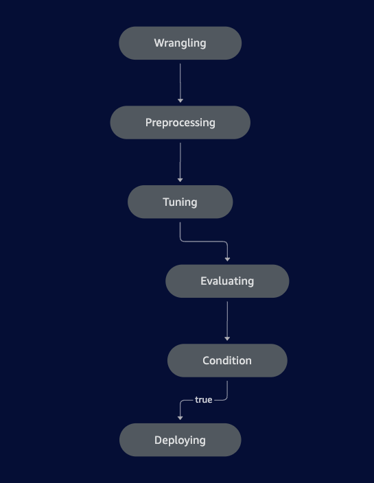
Data Wrangling

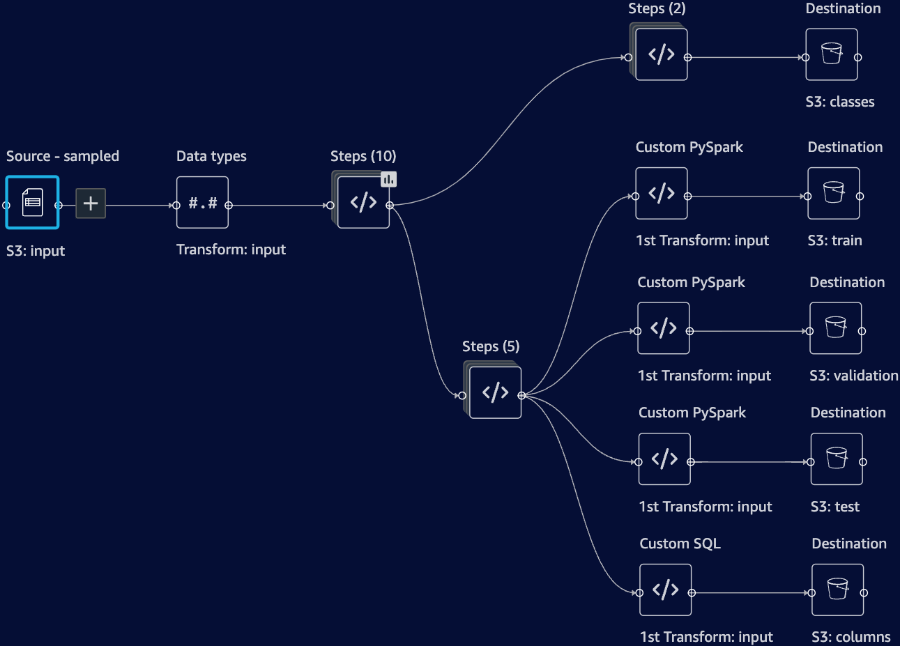
The first step of the pipeline is data preparation (or wrangling) using AWS Data Wrangler, which has its own DAG:

On the first step of the process we’re going to get rid of rarely used web browsers and operating systems, since we will encode all unique values into separate columns and we don’t want to get a very sparse matrix as the result. Another reason for that is due to the nature of the business domain, such outliers often indicate bot traffic or traffic source targeting issues, and should be filtered out.

The histogram for web browsers before applying filtering looks like that:

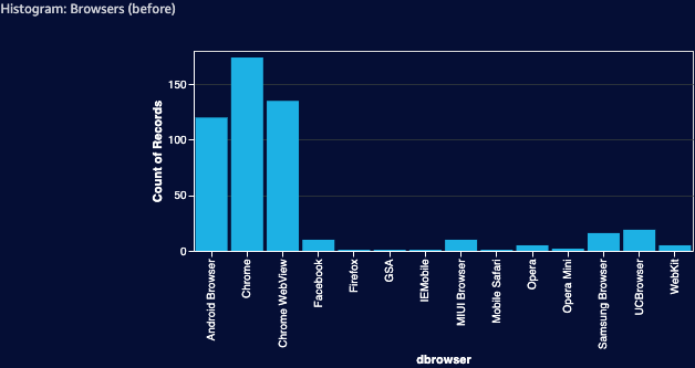
Filtering out web browsers that account for less than 1% of the dataset provides the following result:

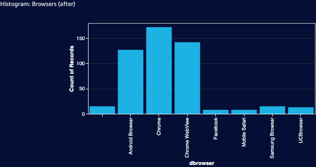
The same applies to countries. Most advertisement campaigns are usually targeted to a specific list of countries and displaying an ad to a user that does not belong to that list will prevent a conversion and will result in wasted money. Low conversion rate can also indicate that the specific campaign is just not very effective in this country, so it makes sense to cut those losses and focus on more promising locations.

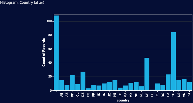
In our case there are quite a few countries that don’t convert much:

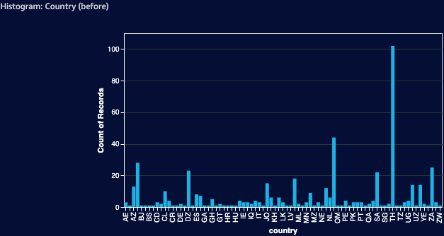
Applying the same 1% filter changes the picture drastically:

The next step is to make sure that categorical columns do not contain any characters that can result in processing errors. To achieve that, we will percent-encode them with a PySpark script:

1
2
3
4
5
6
7
8
9

import urllib
from pyspark.sql.functions import udf
from pyspark.sql.types import StringType

encode_udf = udf(lambda x: urllib.parse.quote(x, safe=''), StringType())

df = df.withColumn('dos', encode_udf('dos'))
df = df.withColumn('dbrowser', encode_udf('dbrowser'))
# Mobile Safari -> Mobile%20Safari

The last step of the common branch of the DAG is to encode categorical columns. In order to train and use an ML model, we need to transform (or encode) non-numerical values to numeric representations. We will use two different approaches for offers and for all other categorical columns that we have. The offers column will be encoded using an indexer, which produces a single column that contains integers, corresponding to a specific offer:

index,offer
0,012a096e-f414-4da7-bbdc-236da34bb545
1,41183105-2ed4-46c6-b654-2f0081aa652d

As for the remaining categorical columns (country, OS, device type and web browser), we will use a one-hot encoding approach, resulting in a new column (with values of 1 or 0) created for each unique value within a category:

country_TH,country_NP,country_BD,country_SA,country_DZ,country_VN,country_US,country_MA,country_ZA,country_MX,country_KE,country_JO,country_AE,country_AZ,country_IN,country_PL,country_ES,country_NG,country_LB,country_CL,country_FR,country_PE,country_NL,country_ID,dos_Android,dos_iOS,dtype_mobile,dtype_tablet,dtype_desktop,dbrowser_Chrome,dbrowser_Chrome%20WebView,dbrowser_Android%20Browser,dbrowser_UCBrowser,dbrowser_Samsung%20Browser,dbrowser_Facebook,dbrowser_Mobile%20Safari

The latitude and longitue columns will remain as is and will be included in the output. The city column will be omitted, because using only latitude and longitue provided similar results in our preliminary research. ISP, network, browser and OS version columns will be removed, since they produce a very sparse model and does not seem to correlate with the offer ID.

At this point we have reached the end of the common branch and the next steps will reflect transformations intended for a specific DAG output.

Data Wrangler Output

The first output that we need is a list of columns. To produce it, we’re just going to limit the number of rows intended for this output to one, so that the processing step won’t have to load a huge dataset file in order to just to get a list of columns in it:

1

SELECT * FROM df TABLESAMPLE(1 ROWS)

The exact same approach is used to get the second output - a list of encoded offers that we created earlier. The only difference is that the output will only contain two columns (index and offer ID) and everything else will be removed.

The last three outputs are samples of our dataset for ML model training, validation and testing. They are created by splitting the dataset in a proportion of 70%, 15% and 15% respectively:

1
2

train, validation, test = df.randomSplit(weights = [0.70, 0.15, 0.15], seed = 13)
df = train

That concludes the process of data preparation and we now approach the next step in our SageMaker pipeline.

Preprocessing

Data Wrangler operates on rows and columns, but in order to execute the next steps, we need to prepare some metadata. Preprocessing step is repsonsible for reading files with offers and columns data from the Data Wrangler output and converting it to JSON that we can reference in our SageMaker pipeline definition script.

Under the hood, it’s just a generic Python environment with various data science libraries pre-installed, that can be used to perform all kinds of data preparation and processing tasks.

Training

Once the data is prepared, we can proceed with training the model. We’re going to use XGBoost and create a model that performs a multiclass classification. In order to account for the fact that our pipeline is automatic and does not involve any manual tuning, we will run a hyperparameter optimization. It will generate several models with different parameters and the best performing model will be deployed to production.

1
2
3
4
5
6
7
8
9
10
11
12
13
14
15
16
17
18
19
20
21
22
23
24
25
26
27
28
29
30
31
32
33
34
35
36
37
38
39
40
41
42
43
44
45
46
47
48
49

xgb_estimator.set_hyperparameters(
    objective="multi:softprob",
        # Multiclass with probabilities
    eval_metric="mlogloss",
        # Negative log-likelihood
        # https://en.wikipedia.org/wiki/Likelihood_function#Log-likelihood
    num_round="100",
        # The number of rounds for boosting
    num_class=JsonGet(
        step_name=step_process.name,
        property_file=classes_map,
        json_path="length_str",
    ),
        # Number of classes
)
xgb_tuner = HyperparameterTuner(
    estimator=xgb_estimator,
    objective_metric_name="validation:mlogloss",
    objective_type="Minimize", # The less log-likelihood is the better
    hyperparameter_ranges={
        # See https://xgboost.readthedocs.io/en/stable/parameter.html
        "alpha": ContinuousParameter(0.01, 10, scaling_type="Logarithmic"),
            # It can be used in case of very high dimensionality so that the algorithm runs faster when implemented.
            # Increasing this value will make model more conservative.
        "eta": ContinuousParameter(0.01, 0.2),
            # It is the step size shrinkage used in update to prevent overfitting.
            # After each boosting step, we can directly get the weights of new features,
            # and eta shrinks the feature weights to make the boosting process more conservative.
        "gamma": ContinuousParameter(0.0, 0.5),
            # A node is split only when the resulting split gives a positive reduction in the loss function.
            # Gamma specifies the minimum loss reduction required to make a split.
            # It makes the algorithm conservative. The values can vary depending on the loss function and should be tuned.
        "min_child_weight": ContinuousParameter(1, 10),
            # It defines the minimum sum of weights of all observations required in a child. It is used to control over-fitting.
            # Higher values prevent a model from learning relations which might be highly specific to the particular sample selected for a tree.
            # Too high values can lead to under-fitting. The larger min_child_weight is, the more conservative the algorithm will be.
        "max_depth": IntegerParameter(3, 10),
            # The maximum depth of a tree. It is used to control over-fitting as higher depth will allow model 
            # to learn relations very specific to a particular sample.
            # Increasing this value will make the model more complex and more likely to overfit.
        "subsample": ContinuousParameter(0.5, 1),
            # It denotes the fraction of observations to be randomly samples for each tree.
            # Setting it to 0.5 means that XGBoost would randomly sample half of the training data prior to growing trees.
            # This will prevent overfitting. Lower values make the algorithm more conservative and prevents overfitting 
            # but too small values might lead to under-fitting.
    },
    max_jobs=10, # Create up to 10 models
    max_parallel_jobs=5, # 5 parallel training job at a time
)

Evaluation

Even with the best performing model at hands, we still want to see if it’s worth deploying it to production. The suitable metric to evaluate a multiclass classification model is a hamming loss - a percentage of samples that were not predicted correctly:

1
2
3
4
5
6
7
8
9
10
11
12
13
14
15
16
17
18
19
20
21
22
23
24

import numpy as np
import pandas as pd
from sklearn.metrics import hamming_loss
import xgboost

# ...

df = pd.read_csv(file_test)
y_test = df.iloc[:, 0].to_numpy()
df.drop(df.columns[0], axis=1, inplace=True)
X_test = xgboost.DMatrix(df.values)

num_class = len(np.unique(y_test))
num_samples = y_test.shape[0]

model = xgboost.Booster()
model.load_model('xgboost-model')

predictions = model.predict(X_test)

predictions = predictions.reshape(num_samples, num_class)
pred_label = np.argmax(predictions, axis=1)

hloss = hamming_loss(y_test, pred_label)

Our pipeline will only proceed with models that have a Hamming loss of 40% or less. Models that don’t fit into that threshold will be discarded and previously deployed model will remaing in production.

Deployment

The last step in the pipeline is model deployment. It is implemented by a Lambda function that loads the model into an S3 bucket that SageMaker inference endpoint uses to access the models, updates the model metadata in a DynamoDB table and performs a cleanup.

Testing

We can now finally call our API and get predictions. The API requires only one parameter - a campaign ID:

curl https://$API_GATEWAY_HOST/predict/97318a5c-bbab-4a5a-8a28-c6ab6fcbd79b

{
  // Model input
  "input": "100.5997,13.5989,1,0,0,0,0,0,0,0,0,0,0,0,0,0,0,0,0,0,0,0,0,0,0,0,1,0,1,0,0,0,1,0,0,0,0,0",
  // Model output
  "output": "[[0.49411922693252563, 0.5058807730674744]]",
  // Predicted offer
  "predicted": {
    "index": 1,
    "offer": "41183105-2ed4-46c6-b654-2f0081aa652d",
    "probability": 0.5058807730674744
  },
  // Analyzed data
  "source": {
    "ip": "16.170.153.144",
    "dos": "Mac OS",
    "dosversion": "10.15.7",
    "dbrowser": "Chrome",
    "dbrowserversion": "98.0.4758.109",
    "isp": "AMAZON-02",
    "network": "16.168.0.0/14",
    "country": "SE",
    "city": "Stockholm",
    "long": 18.0717,
    "lat": 59.3287
  },
  // All predicted offers
  "predictions": [
    { "index": 1, "probability": 0.5058807730674744, "offer": "41183105-2ed4-46c6-b654-2f0081aa652d" },
    { "index": 0, "probability": 0.49411922693252563, "offer": "012a096e-f414-4da7-bbdc-236da34bb545" }
  ],
  // Data to model mappings
  "mappings": {"long":100,"lat":13,"country_TH":1,"country_NP":0,"country_BD":0,"country_SA":0,"country_DZ":0,"country_VN":0,"country_US":0,"country_MA":0,"country_ZA":0,"country_MX":0,"country_KE":0,"country_JO":0,"country_AE":0,"country_AZ":0,"country_IN":0,"country_PL":0,"country_ES":0,"country_NG":0,"country_LB":0,"country_CL":0,"country_FR":0,"country_PE":0,"country_NL":0,"country_ID":0,"dos_Android":1,"dos_iOS":0,"dtype_mobile":1,"dtype_tablet":0,"dtype_desktop":0,"dbrowser_Chrome":0,"dbrowser_Chrome%20WebView":1,"dbrowser_Android%20Browser":0,"dbrowser_UCBrowser":0,"dbrowser_Samsung%20Browser":0,"dbrowser_Facebook":0,"dbrowser_Mobile%20Safari":0},
  // Model metadata
  "endpoint": {
    "campaign": "97318a5c-bbab-4a5a-8a28-c6ab6fcbd79b",
    "model": "3cb70203-a1e4-7f82-b7b4-b8c89bc67305",
    // CSV columns
    "columns": ["long","lat","country_TH","country_NP","country_BD","country_SA","country_DZ","country_VN","country_US","country_MA","country_ZA","country_MX","country_KE","country_JO","country_AE","country_AZ","country_IN","country_PL","country_ES","country_NG","country_LB","country_CL","country_FR","country_PE","country_NL","country_ID","dos_Android","dos_iOS","dtype_mobile","dtype_tablet","dtype_desktop","dbrowser_Chrome","dbrowser_Chrome%20WebView","dbrowser_Android%20Browser","dbrowser_UCBrowser","dbrowser_Samsung%20Browser","dbrowser_Facebook","dbrowser_Mobile%20Safari"],
    // Category encodings
    "classes": {
      "012a096e-f414-4da7-bbdc-236da34bb545": "0",
      "41183105-2ed4-46c6-b654-2f0081aa652d": "1"
    },
    // Model evaluation results
    "evaluation": {
      "hamming_loss": 0.3316062176165803 // Loss rate is 33%
    },
    "modified": 1646122738
  }
}

The model predicted that the current user will most likely convert with offer 41183105-2ed4-46c6-b654-2f0081aa652d and the possibility that this offer is the best for this user compared to other offers is slightly above 50%. The response also contains detailed information about input and output data, as well as the model information.

The API also supports an optional input argument that can be used to provide the model with an input directly, without analyzing the current user’s IP address and user agent string. The input format is a CSV without column names and the order of columns must be the same as described in endpoint.columns field:

curl https://$API_GATEWAY_HOST/predict/97318a5c-bbab-4a5a-8a28-c6ab6fcbd79b?input=100.5997,13.5989,1,0,0,0,0,0,0,0,0,0,0,0,0,0,0,0,0,0,0,0,0,0,0,0,1,0,1,0,0,0,1,0,0,0,0,0

Conclusion

Building a machine learning based system is a complex subject that requires a committed effort of a team of engineers and analysts. The ability to sustain constant evolution is one of the most important traits such system must have in order to succeed. Leveraging modern tools and cloud services designed with this in mind opens up a possibility for even small teams to build powerful and sophisticated ML applications.